13 Priority Queues and Heaps

Priority queue applications

Event-driven simulation.	(customers in a line, colliding particles)
Numerical computation.	(reducing roundoff error)
Data compression.	(Huffman codes)
Graph searching.	(Dijkstra’s algorithm, Prim’s algorithm)
Number theory.	(sum of powers)
Artificial intelligence.	(A* search)
Statistics.	(maintain largest M values in a sequence)
Operating systems.	(load balancing, interrupt handling)
Discrete optimization.	(bin packing, scheduling)
Spam filtering.	(Bayesian spam filter)

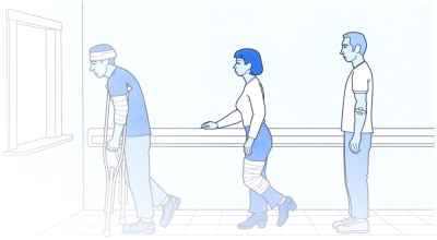
Priority queue

A priority queue is a data structure for maintaining a set S of elements, each with an associated value called a key. There are two kinds of priority queues: max-priority queues and min-priority queues.

Max-priority queue supports the following operations.

Insert(S, x): insert the element x into the set S or S\gets S\cup\{x\}.
Max(S): return the element of S with the largest key.
Remove-Max(S): remove and return the element of S with the largest key.
Increase-Key(S, x, \Delta k): increase the value of element x’s key by the \Delta k.

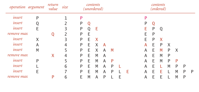
Unordered and ordered array implementation

A sequence of operations on a max-priority queue

Analysis

Challenge: Implement all operations efficiently.

implementation	insert	remove max	max
unordered array	1	N	N
ordered array	N	1	1
goal

13.1 Binary Heaps

Introduction

Max heap: A tree is heap-ordered if the key in each node is larger than or equal to the keys in all of that node’s children (if any)
Min heap: A tree is heap-ordered if the key in each node is smaller than or equal to the keys in all of that node’s children (if any)

Max heap: No node in a heap-ordered tree has a key larger than the key at the root
Min heap: No node in a heap-ordered tree has a key smaller than the key at the root

Binary heap representations

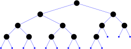
A binary heap data structure is a complete binary tree that can be represented by an array object.

Complete binary tree is perfectly balanced, except for bottom level.
Height of complete binary tree with N nodes is \log_{2}(N+1).
Array representation of a max binary heap.

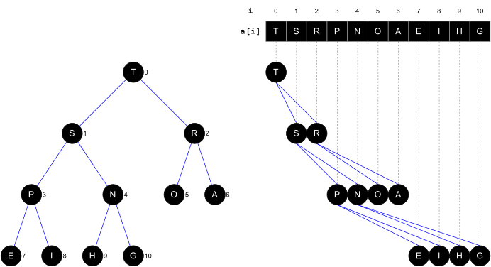
Binary heap properties

Largest key is a[0], which is root of max binary heap.
Can use array indices to move through tree.

function Parent(i)
    return floor((i - 1) / 2)

function LeftChild(i)
    return 2 * i + 1

function RightChild(i)
    return 2 * i + 2

Insert Key

Promotion in a heap

Scenario. Child’s key becomes larger key than its parent’s key. (violation)
To eliminate the violation:
- Exchange key in child with key in parent.
- Repeat until heap order restored.

function Up-Heap(a, i)
    while i > 0 do
        p ← Parent(i)
        if a[i] > a[p] then
            Swap(a, i, p)
            i ← p
        else
            return

Insertion in a heap

Insert.: Add node at end, then percolate it up.
Cost.: At most \log_{2}N+1 compares.

function Insert(a, k)
    n ← a.size
    a[n] ← k
    Up-Heap(a, n)
    a.size ← a.size + 1

Example

Given a max binary heap

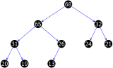
0 1 2 3 4 5 6 7 8 9 10 11

68 65 32 31 26 24 21 20 19 13
Insert key 66 into the heap

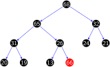
0 1 2 3 4 5 6 7 8 9 10 11

68 65 32 31 26 24 21 20 19 13 \textcolor{red}{66}
Swap 66 and 26

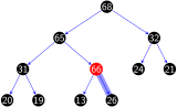
0 1 2 3 4 5 6 7 8 9 10 11

68 65 32 31 \textcolor{red}{66} 24 21 20 19 13 \textcolor{blue}{26}
Swap 66 and 65

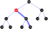
0 1 2 3 4 5 6 7 8 9 10 11

68 \textcolor{red}{66} 32 31 \textcolor{blue}{65} 24 21 20 19 13 \textcolor{blue}{26}

0	1	2	3	4	5	6	7	8	9	10	11
68	65	32	31	26	24	21	20	19	13

0	1	2	3	4	5	6	7	8	9	10	11
68	65	32	31	26	24	21	20	19	13	\textcolor{red}{66}

0	1	2	3	4	5	6	7	8	9	10	11
68	65	32	31	\textcolor{red}{66}	24	21	20	19	13	\textcolor{blue}{26}

0	1	2	3	4	5	6	7	8	9	10	11
68	\textcolor{red}{66}	32	31	\textcolor{blue}{65}	24	21	20	19	13	\textcolor{blue}{26}

Remove Max

Demotion in a heap

Scenario. Parent’s key becomes smaller than one (or both) of its children’s. (vilolation)
To eliminate the violation:
- Exchange key in parent with key in larger child.
- Repeat until heap order restored.

function Down-Heap(a, i)
    l ← LeftChild(i)
    r ← RightChild(i)
    largest ← i

    if l < a.size and a[l] > a[largest] then
        largest ← l

    if r < a.size and a[r] > a[largest] then
        largest ← r

    if largest ≠ i then
        Swap(a, i, largest)
        Down-Heap(a, largest)

Delete the maximum in a heap

Delete max. Exchange root with node at end, then sink it down.
Cost. At most 2\log_{2}N compares.

function Remove-Max(a)
    n ← a.size
    Swap(a, 0, n - 1)
    a.size ← a.size - 1
    Down-Heap(a, 0)
    return a[n]

Example

Given a max binary heap

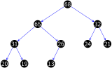
0 1 2 3 4 5 6 7 8 9 10 11

68 65 32 31 26 24 21 20 19 13
Delete max : swap 68 and 13 , delete 68

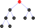
0 1 2 3 4 5 6 7 8 9 10 11

\textcolor{red}{13} 65 32 31 26 24 21 20 19 \textcolor{lightgray}{68}
Swap 13 and 65

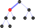
0 1 2 3 4 5 6 7 8 9 10 11

\textcolor{blue}{65} \textcolor{red}{13} 32 31 26 24 21 20 19 \textcolor{lightgray}{68}
Swap 13 and 31

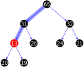
0 1 2 3 4 5 6 7 8 9 10 11

\textcolor{blue}{65} \textcolor{blue}{31} 32 \textcolor{red}{13} 26 24 21 20 19 \textcolor{lightgray}{68}
Swap 13 and 20

0 1 2 3 4 5 6 7 8 9 10 11

\textcolor{blue}{65} \textcolor{blue}{31} 32 \textcolor{blue}{20} 26 24 21 \textcolor{red}{13} 19 \textcolor{lightgray}{68}

0	1	2	3	4	5	6	7	8	9	10	11
68	65	32	31	26	24	21	20	19	13

0	1	2	3	4	5	6	7	8	9	10	11
\textcolor{red}{13}	65	32	31	26	24	21	20	19	\textcolor{lightgray}{68}

0	1	2	3	4	5	6	7	8	9	10	11
\textcolor{blue}{65}	\textcolor{red}{13}	32	31	26	24	21	20	19	\textcolor{lightgray}{68}

0	1	2	3	4	5	6	7	8	9	10	11
\textcolor{blue}{65}	\textcolor{blue}{31}	32	\textcolor{red}{13}	26	24	21	20	19	\textcolor{lightgray}{68}

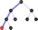
0	1	2	3	4	5	6	7	8	9	10	11
\textcolor{blue}{65}	\textcolor{blue}{31}	32	\textcolor{blue}{20}	26	24	21	\textcolor{red}{13}	19	\textcolor{lightgray}{68}

Analysis

implementation	insert	remove max	max
unordered array	1	N	N
ordered array	N	1	1
binary heap	\log_{2}N	\log_{2}N	1

Increase Key

To increase the value of a certain key inside the max-heap, we need to reach this key first. In ordinary heaps, we can’t search for a specific key inside the heap.
Therefore, we’ll keep a map (hash table) beside the original array. This map will store the index of each key inside the heap.

function Increase-Key(a, k, Δk, map)
    i ← map[k]
    map.Remove(k)
    a[i] ← a[i] + Δk
    map[a[i]] ← i
    Up-Heap(a, i, map)

13.2 d-Heaps

Introduction

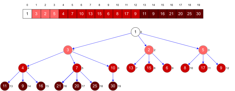
a d-heap is a heap, each node of which has d children.

A min 3-heap

Analysis

A d-heap is much shallower than a binary heap

implementation	insert	remove max	max
unordered array	1	N	N
ordered array	N	1	1
binary heap	\log_{2}N	\log_{2}N	1
d-heap	\log_{d}N	\log_{d}N	1

13.3 Application

Simulation

Molecular dynamics simulation of hard discs

Goal.: Simulate the motion of N moving particles that behave according to the laws of elastic collision.
Problem.: N bouncing balls in the unit square.

Moving particles interact via elastic collisions with each other and walls.
Each particle is a disc with known position, velocity, mass, and radius.
No other forces.

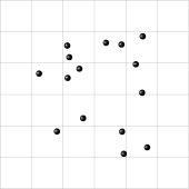
Bouncing balls

Check for balls colliding with each other.
- Physics problems: when? what effect?
- CS problems: which object does the check? too many checks?

Time-driven Simulation

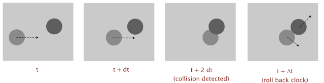
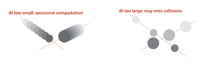
Discretize time in quanta of size dt.

Update the position of each particle after every dt units of time, and check for overlaps.
If overlap, roll back the clock to the time of the collision, update the velocities of the colliding particles, and continue the simulation.

Main drawbacks

\sim N^{2}/2 overlap checks per time quantum.
Simulation is too slow if dt is very small.
May miss collisions if dt is too large. (if colliding particles fail to overlap when we are looking)

Event-driven simulation

Change state only when something happens.

Between collisions, particles move in straight-line trajectories.
Focus only on times when collisions occur.
Maintain \textcolor{blue}{PQ} of collision events, prioritized by time.
Remove the min = get next collision.

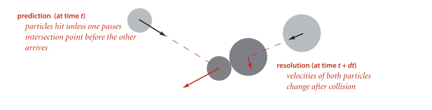
Collision prediction. Given position, velocity, and radius of a particle. When will it collide next with a wall or another particle?

Collision resolution. If collision occurs, update colliding particle(s) according to laws of elastic collisions.

Particle-wall collision

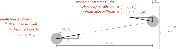
Collision prediction and resolution.

Particle of radius s at position (r_{x},r_{y}).
Particle moving in unit box with velocity (v_{x},v_{y}).
Will it collide with a vertical wall? If so, when?

Particle-particle collision prediction

Collision prediction

Particle i: radius s_{i}, position (rx_{i},ry_{i}), velocity (vx_{i},vy_{i}).
Particle j: radius s_{j}, position (rx_{j},ry_{j}), velocity (vx_{j},vy_{j}).

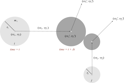
Will particles i and j collide? If so, when? \begin{align} \Delta t & =\begin{cases} \infty & \text{if }\Delta v\Delta r\geq0\\ \infty & \text{if }d<0\\ -\dfrac{\Delta v\Delta r}{\Delta v\Delta v} & \text{otherwise} \end{cases}\\ \sigma & =\sigma_{i}+\sigma_{j}\\d & =(\Delta v\Delta r)^{2}-(\Delta v\Delta v)(\Delta r\Delta r-\sigma^{2}) \end{align} where \begin{align} \Delta v & =(\Delta vx,\Delta vy)=(vx_{i}-vx_{j},vy_{i}-vy_{j})\\ \Delta r & =(\Delta rx,\Delta ry)=(rx_{i}-rx_{j},ry_{i}-ry_{j}) \end{align}

Particle-particle collision resolution

Collision resolution

When two particles collide, how does velocity change?

\begin{array}{ccl} vx_{i}^{\prime} & = & vx_{i}+\dfrac{Jx}{m_{i}}\ \ vy_{i}^{\prime} & = & vy_{i}+\dfrac{Jy}{m_{i}}\ \ vx_{j}^{\prime} & = & vx_{j}-\dfrac{Jx}{m_{j}}\ \ vy_{j}^{\prime} & = & vy_{j}-\dfrac{Jy}{m_{j}} \end{array}

where

\begin{array}{ccl} J & = & \dfrac{2m_{i}m_{j}(\Delta v\Delta r)}{\sigma(m_{i}+m_{j})}\ \ Jx & = & \dfrac{J\Delta rx}{\sigma}\ \ Jy & = & \dfrac{J\Delta ry}{\sigma} \end{array}

Collision system: event-driven simulation main loop

Initialization

Fill PQ with all potential particle-wall collisions. (“potential” since collision may not happen if some other collision intervenes)
Fill PQ with all potential particle-particle collisions.

Main loop

Delete the impending event from PQ (min priority = t).
If the event has been invalidated, ignore it.
Advance all particles to time t, on a straight-line trajectory.
Update the velocities of the colliding particle(s).
Predict future particle-wall and particle-particle collisions involving the colliding particle(s) and insert events onto PQ.

13 Priority Queues and Heaps

Priority queue applications

Priority queue

Unordered and ordered array implementation

Analysis

13.1 Binary Heaps

Introduction

Binary heap representations

Binary heap properties

Insert Key

Promotion in a heap

Insertion in a heap

Example

Remove Max

Demotion in a heap

Delete the maximum in a heap

Example

Analysis

Increase Key

13.2 d-Heaps

Introduction

Analysis

13.3 Application

Simulation

Molecular dynamics simulation of hard discs

Bouncing balls

Time-driven Simulation

Event-driven simulation

Particle-wall collision

Particle-particle collision prediction

Particle-particle collision resolution

Collision system: event-driven simulation main loop

13.4 Workshop

Quiz

Projects

13.5 References