12 B-tree

Introduction

Assumption. So far, search trees were limited to main memory structures \to the dataset organized in a search tree fits in main memory (internal memory)
Problem. Transaction data of a bank > 1 TB per day \to use secondary storage media (HDD, SSD, etc.) (external memory)
Goal. Make a search tree structure secondary-storage-enabled

File system model

Page. Contiguous block of data (e.g., a file or 4,096-byte chunk).
Probe. First access to a page (e.g., from disk to memory).
Property. Time required for a probe is much larger than time to access data within a page.
Cost. Number of probes.
Goal. Access data using minimum number of probes.

B-tree

A B-tree of order M (M \geq 3) invented by Rudolf Bayer and Edward M. McCreight is an M-ary tree with the following properties:

The root is either a leaf or has between 2 and M children.
All nonleaf nodes (except the root) have between \left\lfloor \frac{M+1}{2}\right\rfloor and M children.
- minimum degree m = \left\lfloor \frac{M+1}{2}\right\rfloor
- maximum degree M
All leaves are at the same depth h.
All nodes store keys to guide the searching.

The height of a B-tree

If n\geq1, then for any n-key B-tree T of height h and minimum degree m, h\leq\log_{m}\frac{n+1}{2}

In practice. Number of probes is at most 4.
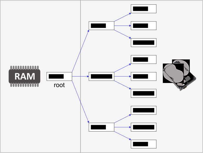
Optimization. Always keep root page in memory.

Structure of Node

Every node x has the following fields:
- x.n, the number of keys currently stored in node x,
- the x.n keys themselves, x.key_{1},x.key_{2},...,x.key_{x.n} stored in nondecreasing order, so that x.key_{1}\leq x.key_{2}\leq...\leq x.key_{x.n}
- x.leaf, a boolean value that is true if x is a leaf and false if x is an internal node.
Each internal node x also contains x.n+1 pointers x.c_{1},x.c_{2},...,x.c_{x.n+1} to its children
The keys x.key_{i} separate the ranges of keys stored in each subtree: if k_{i} is any key stored in the subtree with root x.c_{i}, then k_{1}\leq x.key_{1}\leq k_{2}\leq x.key_{2}\leq...\leq x.key_{x.n}\leq k_{x.n+1}

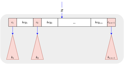
A simple drawing for a B-tree node

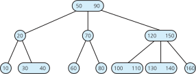
2-3 tree
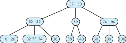
2-3-4 tree

12.1 Basic operations on B-trees

Introduction

We adopt two conventions:

The root of the B-tree is always in main memory, so that a Disk-read on the root is never required; a Disk-Write of the root is required, however, whenever the root node is changed.
Any nodes that are passed as parameters must already have had a Disk-Read operation performed on them.

Searching

function B-Tree-Search(x, k)
    if x.leaf return null
    i ← 1
    while i ≤ x.n and k > x.key_{i}
        i ← i + 1
    if i ≤ x.n and k = x.key_{i}
        return (x, i)
    else
        Disk-Read(x.c_{i})
        return B-Tree-Search(x.c_{i}, k)

Challenge: Can we make any improvement?

Creating an empty B-tree

function B-Tree-Create(T)
    x ← Allocate-Node()
    x.leaf ← true
    x.n ← 0
    Disk-Write(x)
    T.root ← x

There are two kinds of algorithms:

“Single pass down” algorithms that proceed downward from the root of the tree, without having to back up (pre-processing)
“Two-pass” algorithms (post-processing)

They use three kind of actions to maintain the search tree

Split

Merge

Borrow (rotation)

Single-pass Insertion

Splitting a node in a B-tree

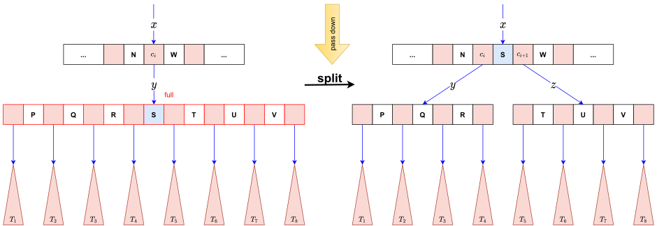
function B-Tree-Split-Child(x, i)
    z ← Allocate-Node()
    y ← x.c_{i}
    z.leaf ← y.leaf
    z.n ← m-1
    for j ← [1,...,m-1]
        z.key_{j} ← y.key_{j+m}
    if not y.leaf
        for j ← [1,...,m]
            z.c_{j} ← y.c_{j+m}
    y.n ← m-1
    for j ← [x.n+1,...,i+1]
        x.c_{j+1} ← x.c_{j}
    x.c_{i+1} ← z
    for j ← [x.n,...,i]
        x.key_{j+1} ← x.key_{j}
    x.key_{i} ← y.key_{m}
    x.n ← x.n+1
    Disk-Write(y)
    Disk-Write(z)
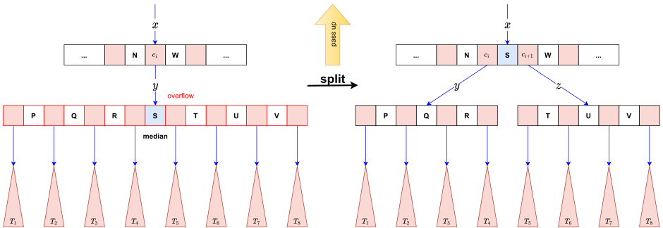
    Disk-Write(x)

B-tree(m=4,M=8): split

Inserting a key into a B-tree

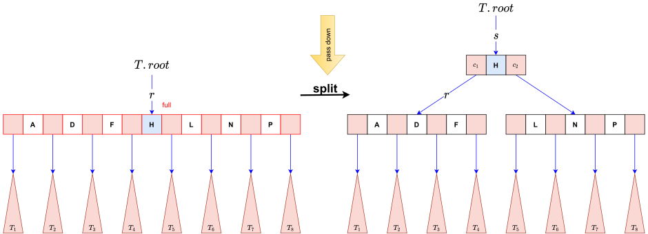
function B-Tree-Insert(T, k)
    r ← T.root
    if r.n = 2m-1
        s ← Allocate-Node()
        T.root ← s
        s.leaf ← false
        s.n ← 0
        s.c_{1} ← r
        B-Tree-Split-Child(s, 1)
        B-Tree-Insert-Nonfull(s, k)
    else
        B-Tree-Insert-Nonfull(r, k)

B-tree(m=4,M=8): split at root

Inserting a key into a B-tree

function B-Tree-Insert-Nonfull(x, k)
    i ← x.n
    if x.leaf
        while i ≥ 1 and k < x.key_{i}
            x.key_{i+1} ← x.key_{i}
            i ← i - 1
        x.key_{i+1} ← k
        x.n ← x.n + 1
        Disk-Write(x)
    else
        while i ≥ 1 and k < x.key_{i}
            i ← i - 1
        i ← i + 1
        Disk-Read(x.c_{i})
        if x.c_{i}.n = 2m - 1
            B-Tree-Split-Child(x, i)
            if k > x.key_{i}
                i ← i + 1
        B-Tree-Insert-Nonfull(x.c_{i}, k)

Example of Insertion

Consider B-tree(m=3,M=6)

Initial tree
B inserted
Q inserted
L inserted
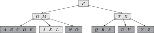
F inserted

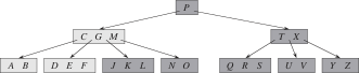
Insertion

Bottom-up Insertion

All insertions start at a leaf node.
If the node contains more than the maximum allowed number of keys, then the node is overflow:
- A single median key is chosen from among the node’s keys
- Keys less than the median are put in the new left node and keys greater than the median are put in the new right node.
- The median is inserted in the node’s parent, which may cause it to be split, and so on. If the node has no parent (i.e., the node was the root), create a new root above this node.

B-tree(m=4,M=7)

Example of Insertion

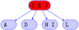
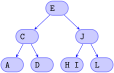
Consider B-tree(m=2,M=3)

Initial tree
I inserted
D inserted

Deletion

Deletion from a leaf node

Delete it from the node.
If underflow happens, rebalance the tree.

Deletion from an internal node: Each key in an internal node acts as a separation value for two subtrees

Choose a new separator (either the largest key in the left subtree or the smallest key in the right subtree), remove it from it is in, and replace the key to be deleted with the new separator.

Rebalancing after deletion

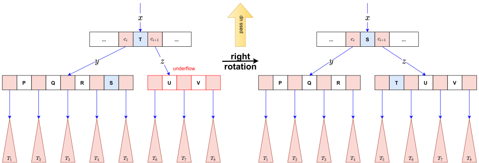
If the deficient node’s right sibling exists and has more than the minimum number of elements, then rotate left
Otherwise, if the deficient node’s left sibling exists and has more than the minimum number of elements, then
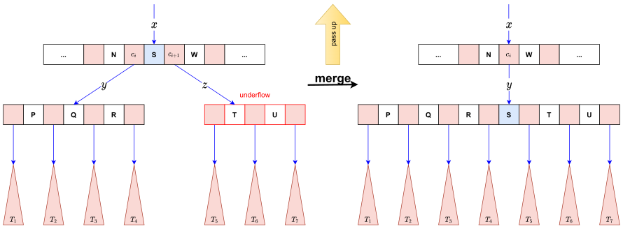
Otherwise, if both immediate siblings have only the minimum number of elements, then merge with a sibling sandwiching their separator taken off from their parent.

Right rotation

B-tree(m=4,M=7)

Merge

B-tree(m=4,M=7)

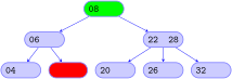
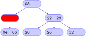
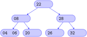
Example of Deletion

Consider B-tree(m=2,M=3)

Initial tree
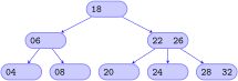
24 deleted
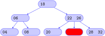
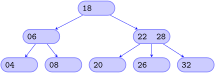
18 deleted

12.2 Applications

Indexing

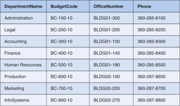
Indexing is a data structure technique to efficiently retrieve records from the database files based on some attributes on which the indexing has been done.

Indexing can be

Primary Index: primary key
Secondary Index: candidate key
Clustering Index: non-key

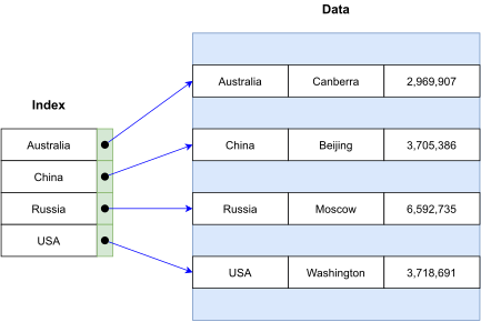
Dense Index

In dense index, there is an index record for every search key value in the database. This makes searching faster but requires more space to store index records itself. Index records contain search key value and a pointer to the actual record on the disk.

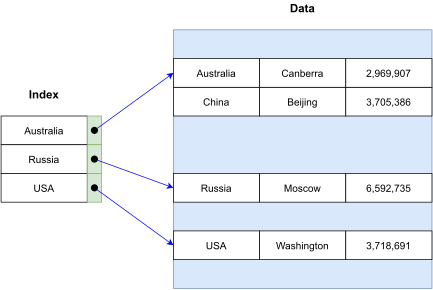
Sparse Index

In sparse index, index records are not created for every search key.

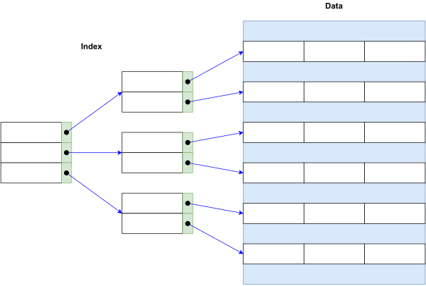
Multilevel Index

Multi-level Index helps in breaking down the index into several smaller indices in order to make the top level so small that it can be saved in a single disk block, which can easily be accommodated anywhere in the main memory.

B-tree variants

B+ tree is a B-tree:

Copies of the keys are stored in the internal nodes.
The keys and records are stored in leaves.
In addition, a leaf node may include a pointer to the next leaf node to speed sequential access.

B* tree is a B-tree that ensures non-root nodes are at least 2/3 full instead of 1/2.

Searching a B+ Tree

Table people

ID	name	age
1	Peter	20
2	Mary	30
3	John	25
…	…	…

Queries

SELECT name
FROM people
WHERE age = 25

Exact key values:

Start at the root
Proceed down, to the leaf

SELECT name
FROM people
WHERE 20 <= age AND age <= 30

Range queries:

As above
Then sequential traversal

Applications

B-trees (and variants) are widely used for file systems and databases.

Windows: NTFS.
Mac: HFS, HFS+.
Linux: ReiserFS, XFS, Ext3FS, JFS.
Databases: ORACLE, DB2, INGRES, SQL, PostgreSQL.

12.3 Workshop

Quiz

What is a B-tree?
What is Indexing?

12 B-tree

Introduction

File system model

B-tree

The height of a B-tree

Structure of Node

12.1 Basic operations on B-trees

Introduction

Searching

Creating an empty B-tree

Single-pass Insertion

Splitting a node in a B-tree

Inserting a key into a B-tree

Inserting a key into a B-tree

Example of Insertion

Insertion

Bottom-up Insertion

Example of Insertion

Deletion

Right rotation

Merge

Example of Deletion

12.2 Applications

Indexing

Dense Index

Sparse Index

Multilevel Index

B-tree variants

B-tree variants

Searching a B+ Tree

Applications

12.3 Workshop

Quiz

Projects

12.4 References