4  Dynamic Programming

4.1 Dynamic Programming

Problems in Recursion

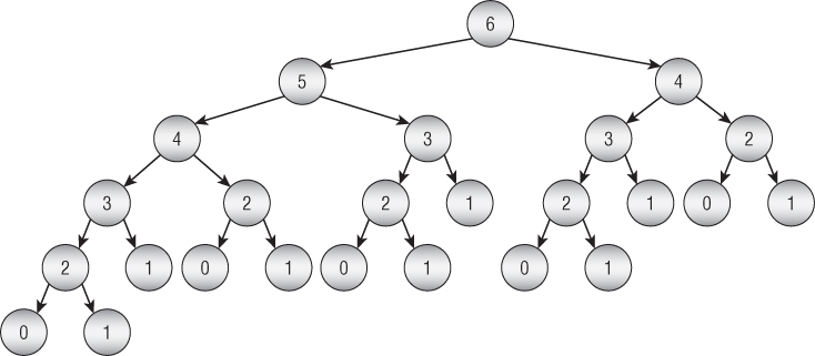
• The number of terms computed by the recursive algorithm for determining the nth Fibonacci term is exponential in n

  int fibonacci(int n)  { 
      if(n <= 1)
          return 1;
      else
          return fibonacci(n-1) + fibonacci(n-2);
  } 

• The figure shows the Fibonacci algorithm’s call tree when it evaluates fibonacci(6)

Dynamic Programming

Dynamic programming is a method for solving complex problems by breaking them down into simpler, overlapping subproblems, solving each subproblem only once, and storing their solutions for future use.

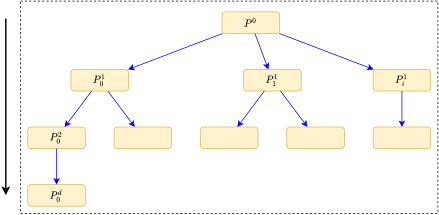
• Dynamic programming is similar to divide-and-conquer in that an instance of a problem is divided into smaller instances.

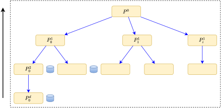
• However, in this approach we solve small instances first, store the results, and later, whenever we need a result, look it up instead of recomputing it.

• Dynamic programming is a bottom-up approach

int fibonacci(int n) {
    int f[100];

    f[0] = 1;
    f[1] = 1;
    for (int i = 2; i <= n; i++)
        f[i] = f[i - 1] + f[i - 2];
    return f[n];
}

The Binomial Coefficient

• The binomial coefficient is given by \begin{equation} \binom{n}{k}=\frac{n!}{k!(n-k)!}\quad\text{for}\quad0\leq k\leq n \end{equation}

• We have recursive formula \begin{equation} \binom{n}{k}=\begin{cases} 1 & k=0\text{ or }k=n\\ \binom{n-1}{k-1}+\binom{n-1}{k} & 0<k<n \end{cases} \end{equation}

Recursive solution

The recursive function below calculates the binomial coefficient by directly applying the recursive formula.

int bin(int n, int k) {  
    if ( k == 0 || k == n)
        return 1;
    else
        return bin(n-1, k - 1) + bin(n - 1, k);
}

• This algorithm is very inefficient.

DP solution

• We define an array B[i][j] containing \binom{i}{j}

1. Establish a recursive property. \begin{equation} B[i][j]=\begin{cases} 1 & j=0\text{ or }j=i\\ B[i-1][j-1]+B[i-1][j] & 0<j<i \end{cases} \end{equation}

2. Solve an instance of the problem in a bottom-up fashion by computing the rows in B in sequence starting with the first row.

int bin(int n, int k) {  
    int B[1000][100];

    for (int i = 0; i <= n; i++) {
        for (int j = 0; j <= i; j++) {
            if (j == 0 || j == i)
                B[i][j] = 1;
            else
                B[i][j] = B[i-1][j-1] + B[i-1][j];
        }
    }
    return B[n][k];
}

4.2 Optimization Problems

Principle of Optimality

A problem is said to satisfy the Principle of Optimality if the subsolutions of an optimal solution of the problem are themesleves optimal solutions for their subproblems.

• In practice, it is necessary to show that the principle applies before assuming that an optimal solution can be obtained using dynamic programming.

Longest Path Problem

Finding the longest simple paths from each vertex to all other vertices.

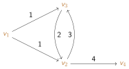
• The optimal (longest) simple path from v_{1} to v_{4} is {v_{1} \to v_{3} \to v_{2} \to v_{4}}.
• However, the subpath {v_{1} \to v_{3}} is not an optimal (longest) path from v_{1} to v_{3}

Dynamic Programming

1. Establish a recursive property that gives the optimal solution to an instance of the problem.
2. Compute the value of an optimal solution in a bottom-up fashion.
3. Construct an optimal solution in a bottom-up fashion.

Chained Matrix Multiplication

• Multiply a 2\times3 matrix times a 3\times4 matrix, the resultant matrix is a 2\times4 matrix \left[\begin{array}{ccc} 1 & 2 & 3\\ 4 & 5 & 6 \end{array}\right]\left[\begin{array}{cccc} 7 & 8 & 9 & 1\\ 2 & 3 & 4 & 5\\ 6 & 7 & 8 & 9 \end{array}\right]=\left[\begin{array}{cccc} 29 & 35 & 41 & 38\\ 74 & 89 & 104 & 83 \end{array}\right] the total number of elementary multiplication is 2\times3\times4=24.

• In general, to multiply an m\times n matrix times a n\times p matrix using the standard method, it is necessary to do \begin{equation} m\times n\times p\quad\text{elementary multiplications} \end{equation}

• Consider the multiplication of the following four matrices:

\underset{20\times2}{\underbrace{A}}\times\underset{2\times30}{\underbrace{B}}\times\underset{30\times12}{\underbrace{C}}\times\underset{12\times8}{\underbrace{D}}

• Matrix multiplication is an associative operation, meaning that the order in which we multiply does not matter. There are five different orders in which we can multiply four matrices, each possibly resulting in a different number of elementary multiplications. \begin{array}{lll} A(B(CD)) & 30\times12\times8+2\times30\times8+20\times2\times8 & =3680\\ (AB)(CD) & 20\times2\times30+30\times12\times8+20\times30\times8 & =8880\\ A((BC)D) & 2\times30\times12+2\times12\times8+20\times2\times8 & =1232\\ (AB)C)D & 20\times2\times30+20\times30\times12+20\times12\times8 & =10320\\ (A(BC))D & 2\times30\times12+20\times2\times12+20\times12\times8 & =3120 \end{array}

Multiply n matrices: A_{1},A_{2},\ldots,A_{n}.

• It is not hard to see that the principle of optimality applies in this problem.

Let

• d_{0} be the number of rows in A_{1} and

• d_{k} be the number of columns in A_{k} for 1\leq k\leq n, the dimension of A_{k} is d_{k-1}\times d_{k}

Solution to Chained Matrix Multiplication

• Let M[i][j] = minimum number of multiplications needed to multiply A_{i} through A_{j}, if i\leq j.

• Principle of optimality \begin{equation} \begin{array}{lll} M[i][i] & = & 0\\ M[i][j] & = & \min_{i\leq k\leq j-1}\left(M[i][k]+M[k+1][j]+d_{i-1}d_{k}d_{j}\right)\quad\text{if }i<j \end{array} \end{equation}

• Consider the multiplication of the following six matrices \underset{5\times2}{\underbrace{A_{1}}}\times\underset{2\times3}{\underbrace{A_{2}}}\times\underset{3\times4}{\underbrace{A_{3}}}\times\underset{4\times6}{\underbrace{A_{4}}}\times\underset{6\times7}{\underbrace{A_{5}}}\times\underset{7\times8}{\underbrace{A_{6}}} we have d_{0}=5,d_{1}=2,d_{2}=3,d_{3}=4,d_{4}=6,d_{5}=7,d_{6}=8

• The table M is:

  	1	2	3	4	5	6
  1	0	30	64	132	226	348
  2		0	24	72	156	268
  3			0	72	198	366
  4				0	168	392
  5					0	336
  6						0

4.3 Workshop

Quiz

1. What is the dynamic programming?

Exercises

• Write a program

4.4 References