5 ANALYSIS OF ALGORITHM
5.1 Introduction
Analysis of Algorithms
Definition: Analysing an algorithm means predicting the resources that the algorithm requires.
- Time Complexity: How long it takes the algorithm to run
- Space Complexity: The extra memory space the algorithm needs besides the input data itself.
Why Analyze Algorithms?
- Comparison: To compare different algorithms and choose the most efficient one for a given task.
- Optimization: To optimize an algorithm.
- Predictability: To predict how an algorithm will behave with different input sizes and under various conditions.
- Resource Management: To ensure algorithms are efficient in terms of computational resources, such as CPU time and memory.
Methods of Analysis
There are two methods of analysis:
- Empirical analysis
- Theoretical analysis
Time Complexity
Definition: The time complexity of an algorithm estimates how much time the algorithm will use given an input.
\text{time complexity} = T(\text{input size})
Input size depends on the problem’s input data:
- Number of items in the input.
- Total number of bits needed to represent the input.
- Sometimes described by two or more numbers.
Time complexity measures how many basic operations are executed, rather than direct time in seconds.
Definition: Basic Operations can be:
- Machine operations: assignments, arithmetic operations, etc.
- Human operations: move, carry, etc.
- General operations.
Space Complexity
Definition: The space complexity of an algorithm estimates the amount of extra memory space the algorithm needs to perform its operations on an input data.
\text{space complexity} = T(\text{input size})
Example: Maximum Subarray Sum
- Given an array of n numbers, calculate the maximum subarray sum (largest possible sum of a sequence of consecutive values).
- An empty subarray is allowed, so the sum is at least 0.
Example array:

Maximum sum (10):

Algorithm 1
Go through all possible subarrays, calculate the sum of each, and maintain the maximum.
int best = 0;
for (int a = 0; a < n; a++) {
    for (int b = a; b < n; b++) {
        int sum = 0;
        for (int k = a; k <= b; k++) {
            sum += array[k];
        }
        best = max(best, sum);
    }
}
cout << best << "\n";
Algorithm 2
Optimize Algorithm 1 by calculating the sum as the right end of the subarray moves.
int best = 0;
for (int a = 0; a < n; a++) {
    int sum = 0;
    for (int b = a; b < n; b++) {
        sum += array[b];
        best = max(best, sum);
    }
}
cout << best << "\n";
Algorithm 3
Calculate the maximum subarray sum for each ending position from left to right.
- The subarray only contains the element at position k.
- The subarray consists of a subarray ending at k-1 followed by the element at k.
int best = 0, sum = 0;
for (int k = 0; k < n; k++) {
    sum = max(array[k], sum + array[k]);
    best = max(best, sum);
}
cout << best << "\n";
5.2 Types Of Problem
Definitions
- Decision Problem: A problem with a yes or no answer (e.g., “is this number prime?”).
- Search Problem: Requires identifying a solution from a set of possible solutions (e.g., “finding a path”).
- Counting Problem: Requires the total number of solutions to a search problem (e.g., “how many primes in first 100 integers?”).
- Optimization Problem: Requires identifying the best solution to a search problem (e.g., “finding the shortest path”).
Tractable & Intractable Problems
- Tractable: A problem that can be solved in polynomial time.
- Intractable: A problem where execution time grows too quickly for polynomial time solutions (e.g., Travelling Salesperson Problem).
Approximate Solutions
- Heuristic Algorithm: Produces usable solutions in reasonable (polynomial) time. These may not be optimal but are “good enough”.
Decidable/Undecidable Problems
- Uncomputable Problems: Problems that cannot be solved by algorithms even with unlimited time.
- Undecidable: A decision problem that is uncomputable.
The Halting Problem: Given a program code and input, is it possible to tell if it will halt or loop forever without running it?
Complexity Classes
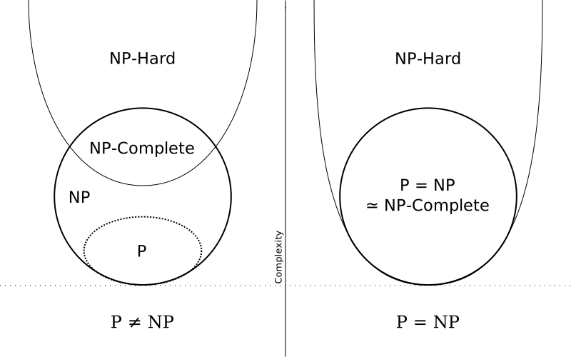
- P: Decision problems solvable in polynomial time on a deterministic machine.
- NP: Decision problems whose positive solutions can be verified in polynomial time.
- NP-complete: A problem in NP such that every problem in NP is reducible to it in polynomial time.
- NP-hard: Satisfies the reduction property of NP-complete, but might not be in NP.
Some NP-complete Problems
- Clique problem
- n-Queens completion
- Boolean satisfiability problem
- Subset sum problem
- Traveling salesman problem
P = NP?
The question of whether P = NP remains unsolved.
5.3 Asymptotic Notation
Big O Notation
History:
- Symbol O introduced by Paul Bachmann in 1894.
- o notation introduced by Edmund Landau in 1909.
- Popularized in CS by Donald Knuth in the 1970s.
Definition: O(g(n)) = \{f(n) : \exists c, n_0 > 0 \text{ s.t. } 0 \leq f(n) \leq cg(n) \forall n \geq n_0\}.
- Represents the upper bound on growth rate.
- Pronounced “big-oh of g of n”.
| Name | Order-of-growth function |
|---|---|
| constant | 1 |
| logarithm | \log n |
| linear | n |
| n-log-n | n \log n |
| quadratic | n^2 |
| cubic | n^3 |
| exponential | 2^n |
| permutation | n! |
Examples
Example: Prove T(n) = 2n^4 + 3n^3 + 5n^2 + 2n + 3 = O(n^4).
Proof. For n \geq 1:
2n^4 + 3n^3 + 5n^2 + 2n + 3 \leq (2+3+5+2+3)n^4 = 15n^4.
Theorem: If T(n) = a_0 + a_1n + ... + a_dn^d (a_d > 0), then T(n) = O(n^d).
Examples: Find the order-of-growth:
- 5n^2 + 3n \log n + 2n + 5 \to O(n^2)
- 20n^3 + 10n \log n + 5 \to O(n^3)
- 3 \log n + 2 \to O(\log n)
- 2^{n+2} \to O(2^n)
- 2n + 100 \log n \to O(n)
Exercises:
If f is in O(g), what can we say about af+b?
If f_{1} and f_{2} are in O(g), what can we say about f_{1}+f_{2}?
If f_{1} is in O(g) and f_{2} is in O(h), what can we say about f_{1}+f_{2}?
If f_{1} is in O(g) and f_{2} is O(h), what can we say about f_{1}\cdot f_{2}?
Big Omega (\Omega) Notation
Definition: \Omega(g(n)) = \{f(n) : \exists c, n_0 > 0 \text{ s.t. } f(n) \geq cg(n) \forall n \geq n_0\}.
- Represents a lower bound on growth rate.
Big Theta (\Theta) Notation
Definition: \Theta(g(n)) = \{f(n) : \exists c_1, c_2, n_0 > 0 \text{ s.t. } c_1g(n) \leq f(n) \leq c_2g(n) \forall n \geq n_0\}.
- Represents an exact growth rate (upper and lower limits).
5.4 Mathematical Techniques
Summation Formulas
- Arithmetic Series: \sum_{k=1}^{n} k = \frac{1}{2}(n^2 + n)
- Sum of Squares: \sum_{k=1}^{n} k^2 = \frac{1}{6}(2n^3 + 3n^2 + n)
- Sum of Cubes: \sum_{k=1}^{n} k^3 = \frac{1}{4}(n^4 + 2n^3 + n^2)
- Geometric Series: \sum_{k=0}^{n} r^k = \frac{1-r^{n+1}}{1-r}
- Harmonic Series: 1 + \frac{1}{2} + ... + \frac{1}{n} \approx \ln n
Generating Functions
Definition: For a sequence \{a_k\}, the Ordinary Generating Function (OGF) is: A(z) = \sum_{k \geq 0} a_k z^k
Common Generating Functions
| Series | Generating Function |
|---|---|
| 1, 1, 1, 1, ... | \frac{1}{1-z} |
| 0, 1, 2, 3, ... | \frac{z}{(1-z)^2} |
| 1, c, c^2, c^3, ... | \frac{1}{1-cz} |
| 1, 1, \frac{1}{2!}, \frac{1}{3!}, ... | e^z |
| 0, 1, \frac{1}{2}, \frac{1}{3}, ... | \ln \frac{1}{1-z} |
Solving Recurrences with Generating Functions
Example: a_n = 5a_{n-1} - 6a_{n-2} with a_0 = 0, a_1 = 1.
- Multiply by z^n and sum: A(z) - z = 5zA(z) - 6z^2A(z).
- Solve for A(z): A(z) = \frac{z}{1-5z+6z^2} = \frac{1}{1-3z} - \frac{1}{1-2z}.
- Result: a_n = 3^n - 2^n.
5.5 Algorithm Analysis
Performance Scenarios
- Best-case: Fastest completion for any input.
- Average-case: Expected complexity over all inputs.
- Worst-case: Slowest completion (guaranteed upper bound).
Complexities for Simple Statements
- Sequential (P_1, P_2): T(n) = T_1(n) + T_2(n)
- Branch (if-else): T(n) = \max(T_1(n), T_2(n))
- Loop: T(n) = \sum_{i} T_i(n)
Examples
Linear Search (Worst Case)
int LinearSearch(int n, int a[], int key) {
    int i = 0;
    while (i < n) {
        if (a[i] == key) return i;
        i++;
    }
    return -1;
}
Complexity: O(n)
Bubble Sort (Worst Case)
void BubbleSort(int n, int a[]) {
    for (int i = 0; i <= n - 2; i++)
        for (int j = n - 1; j >= i + 1; j--)
            if (a[j] < a[j - 1])
                swap(a[j], a[j-1]);
}
Complexity: O(n^2)
Recursive Function Analysis
Steps:
- Identify the Recurrence Relation (Base Case and Recursive Case).
- Write the Relation (e.g., T(n) = T(n-1) + C).
- Solve (Substitution, Recursion Tree, or Master Theorem).
Factorial Example
int factorial(int n) {
    if (n == 0) return 1;
    else return (n * factorial(n - 1));
}
Complexity:
T(n) = T(n-1) + C \implies O(n)
Merge Sort Example
void mergeSort(int a[], int left, int right) {
    if (left < right) {
        int mid = (left + right) / 2;
        mergeSort(a, left, mid);
        mergeSort(a, mid + 1, right);
        merge(a, left, mid, right);
    }
}
Complexity:
T(n) = 2T(n/2) + Cn \implies O(n \log n)
5.6 The Master Theorem
The Master Theorem is a method used to determine the time complexity of divide and conquer algorithms. It provides a solution for recurrence relations of the form
\begin{equation} T\left(n\right)=\left\{ \begin{array}{cc} 1 & n=1\\ a\cdot T\left(\frac{n}{b}\right)+f(n) & n>1 \end{array}\right. \end{equation}
n is the size of the input.
a\geq1 is the number of subproblems in the recursion.
n/b (b>1) is the size of each subproblem. All subproblems are assumed to have the same size.
f(n) is the cost of the work done outside the recursive call, which includes the cost of dividing the problem and the cost of merging the solutions.
Cases:
- Case 1: f(n) = O(n^{\log_b a - \epsilon}) \implies T(n) = \Theta(n^{\log_b a}) (Recursive work dominates).
- Case 2: f(n) = \Theta(n^{\log_b a}) \implies T(n) = \Theta(n^{\log_b a} \log n) (Balanced).
- Case 3: f(n) = \Omega(n^{\log_b a + \epsilon}) \implies T(n) = \Theta(f(n)) (Non-recursive work dominates).
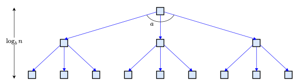
First, consider an algorithm with a recurrence of the form T(n)=aT\left(\frac{n}{b}\right)
- The tree has a depth of \log_{b}n and depth i contains a^{i} nodes. So there are a^{\log_{b}n}=n^{\log_{b}a} leaves, and hence the runtime is \Theta(n^{\log_{b}a}).
Examples
- T(n) = 4T(n/2) + n \implies O(n^2) (Case 1)
- T(n) = 4T(n/2) + n^2 \implies O(n^2 \log n) (Case 2)
- T(n) = 4T(n/2) + n^3 \implies O(n^3) (Case 3)
- T(n) = 2T(n/2) + n \log n \implies O(n \log^2 n)
5.7 Workshop
Quiz
- What is analysis of algorithms?
Exercises
Find the complexities of:
for(i = 0; i < n; i++)
    for (j = 0; j < n; j++)
        b[i][j] += c;

for(i = 0; i < n; i++)
    for (j = i+1; j < n; j++)
b[i][j] -= c;for(i = 0; i < n; i++)
for (j = 0; j < n; j++)
a[i][j] = b[i][j] + c[i][j];for(i = 0; i < n; i++)
for (j = 0; j < n; j++)
for(k = a[i][j] = 0; k < n; k++)
a[i][j] += b[i][k] + c[k][j];Recurrence: T(n) = T(n/2) + 1 and T(n) = 2T(n/2) + \log n.
Tower of Hanoi Complexity.
void HanoiTower(int n, int a, int b, int c) {
    if (n > 0) {
        HanoiTower(n - 1, a, c, b);
        cout << "move from " << a << " to " << c << endl;
        HanoiTower(n - 1, b, a, c);
    }
}- Permutation Complexity.
void Permute(int k, int n, int a[]) {
    if (k == 0) {
        for (int i = 0; i < n; i++) cout << a[i] << " ";
        cout << endl;
    } else {
        for (int i = 0; i < k; i++) {
            swap(a[i], a[k - 1]);
            Permute(k - 1, n, a);
            swap(a[i], a[k - 1]);
        }
    }
}