11 Balanced Binary Search Tree

11.1 Balanced Tree

Introduction

Balance may be defined by:

Comparing the numbers of nodes of the two subtrees
Height balancing: comparing the heights of the twosub trees
Null-path-length balancing: comparing the null-path-length of each of the two sub-trees
Weight balancing: comparing the number of null sub-trees in each of the two sub trees

A binary tree is balanced if the difference in the numbers of nodes of both subtrees of any node in the tree either zero or one.

A binary tree is height-balanced if the difference in height of both subtrees of any node in the tree either zero or one.

A complete binary tree is is height-balanced

Rotations

A rotation allows us to interchange the role of the root and one of the root’s children in a tree while still preserving the BST ordering among the keys in the nodes.
There are two kinds of rotations: right rotation and left rotation

Right rotation

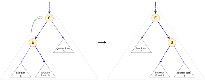
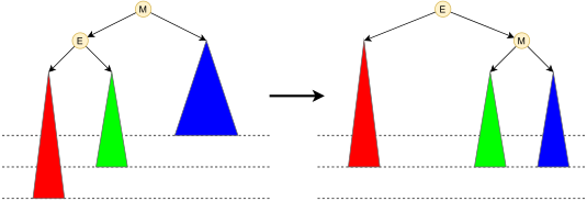
A right rotation involves the root and the left child. The rotation puts the root on the right, essentially reversing the direction of the left link of the root:

Before the rotation, it points from the root to the left child
After the rotation, it points from the old left child (the new root) to the old root (the right child of the new root)

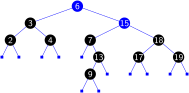
Example

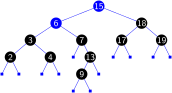
Make right rotation at 15

Implementation

void rightRotate(link& h) {
    link x = h->left; 
    h->left = x->right; 
    x->right = h;
    h = x;
}

Left rotation

A left rotation involves the root and the right child.

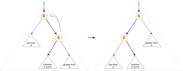
Implementation

void leftRotate(link& h) {
    link x = h->right; 
    h->right = x->left; 
    x->left = h; 
    h = x;
}

Strategies in Balancing Tree

Global rebalancing: an approach to producing better balance in BSTs is periodically to rebalance them explicitly.
- costs at least linear time in the size of the tree
Local rebalancing: balancing BSTs after each operation (insert, delete)

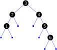
DSW algorithm

The algorithm was proposed by Colin Day and later improved by Quentin F. Stout and Bette L. Warren. Idea of algorithm:

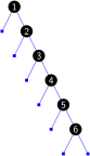
Transform an arbitrary BST into a linked-list-like-tree called backbone or vine by rotations
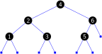
Transform this tree into a perfectly balanced tree by rotations

function CreateBackbone(root)
    p ← root
    while p ≠ null
        if p has a left chid
            make right rotation at p 
        else
            p ← p->right

function CreateCompleteTree(root)
    n ← the number of nodes
    m ← 2^(floor(log_2(n+1))) - 1
    repeat n-m: rotate left and slide down starting from the top
    while (m>1)
        m ← m/2
        repeat m: rotate left and slide down starting from the top

Illustration

BST
Backbone
Perfect

11.2 AVL Tree

AVL Tree

AVL tree

proposed by two Soviet scientists G. M. Adelson-Velskii and E. M. Landis
is BST tree which is height-balanced

\forall p:\left|\boldsymbol{height}(\boldsymbol{LeftSubtree}(p))-\boldsymbol{height}(\boldsymbol{RightSubtree}(p))\right|\le1

The Height of an AVL Tree

Consider the worst case,

To determine the maximum height that an AVL tree with N nodes can have, we can instead ask what is the minimum number of nodes that an AVL tree of height h can have (called AVL tree F_{h}).
We have the recurrence relation

|F_{h}|=|F_{h-1}|+|F_{h-2}|+1 where |F_{0}|=1 and |F_{1}|=2
Solve the equation, we have

|F_{h}|+1\approx\frac{1}{\sqrt{5}}\left[\frac{1+\sqrt{5}}{2}\right]^{h+2}
The height of an AVL tree in the worst case

h\approx1.44\log_{2}|F_{h}|=1.44\log_{2}N

Rebalancing technique

After an insertion/deletion, we may find a node whose new balance violates the AVL condition.
Four cases: LL imbalance, LR imbalance, RR imbalance, RL imbalance
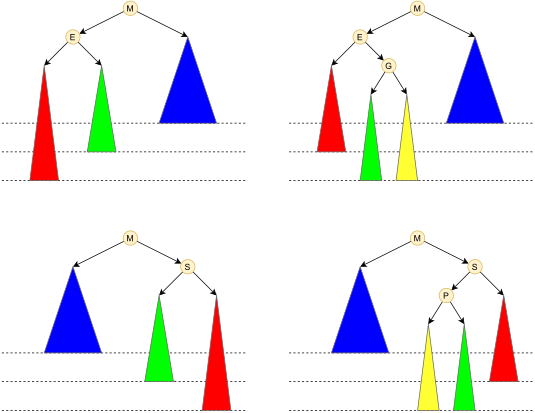
Case LL imbalance is corrected by executing a single right rotation at the node with the imbalance.
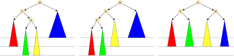
Case LR imbalance is corrected by executing a double rotations

Insertion

function Insert(root,key) 
    if root = null
        root ← new NODE(key)
        return

    if root->key = key 
        return

    if root->key < key 
        Insert(root->right,key)

    if root->key > key 
        Insert(root->left,key)

    if unbalanced at root? rebalance at root

Illustration

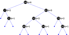
An AVL tree
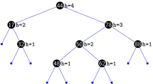
Insert node 54 into the tree \to node 78 become unbalanced
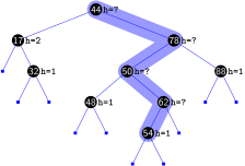
Case RL imbalance \to rebalance by making double rotations

Deletion

Illustration

An AVL tree
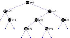
Delete node 32 from the tree \to node 44 become unbalanced
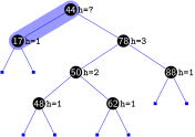
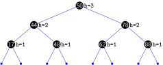
Case RL imbalance \to rebalance by making double rotations

11.3 Red-Black Tree

Red-Black Tree

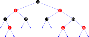
A red–black (RB) tree is a special type of binary search tree that must statsify

Each node is either red or black.
The root is black. (sometimes omitted)
If a node is red, then both its children are black.
Every path from a given node to any of its descendant null link has the same number of black nodes (balance criteria).

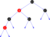
A left-leaning red–black (LLRB) tree (leveraging Andersson’s idea AA tree) is a variant of the red–black tree that has only left red children

Example

A red–black tree
A left-leaning red–black tree
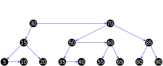
AA tree

The Height of a RB Tree

The height of a red-black BST with N nodes is no more than 2\log_{2}N. It means that the height of an RB tree in the worst case

h\leq2\log_{2}N

Operations

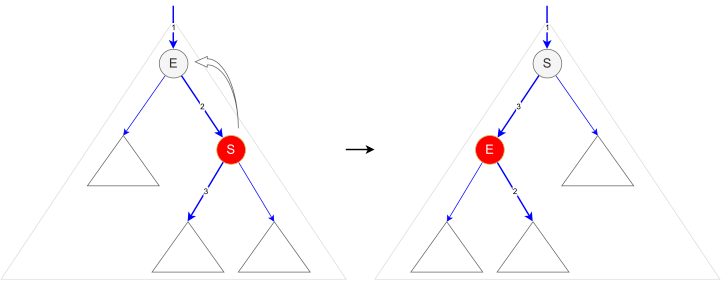
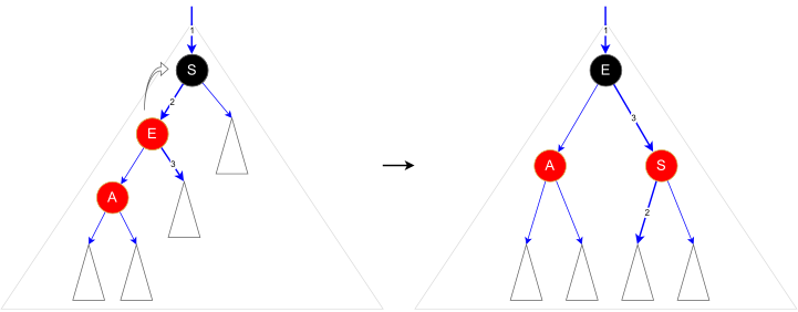
Case 1: Left rotation to orient a right red node to left red node.
Case 2: Right rotation.
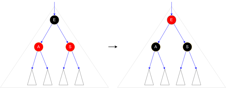
Case 3: Color flip.

Insertion

function Insert(root,key) 
    if root = null
        root ← new NODE(key) # root is red
        return

    if root->key = key 
        return

    if root->key < key 
        Insert(root->right,key)

    if root->key > key 
        Insert(root->left,key)

    if IsRed(root->right) and IsBlack(root->left) RotateLeft(root)
    if IsRed(root->left) and IsRed(root->left->left) RotateRight(root)
    if IsRed(root->left) and IsRed(root->right) FlipColors(root)

Example

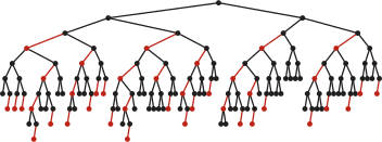
Typical left-leaning red-black BST built from random keys

Illustration

A left-leaning red–black tree
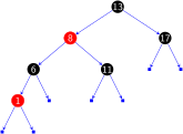
Insert node 7 into the tree
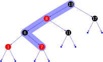
Flip color at 6 into the tree
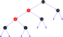
Right rotation at 13 into the tree
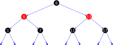
Flip color at root and change root to black color

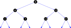
Deletion

Cost summary for symbol-table implementations

implementation	search (worst)	insert (worst)	remove (worst)	search hit (avg)	insert (avg)	remove (avg)	key
unordered list	N	1	N	N/2	1	N/2	equal
ordered list	N	N	N	N/2	N/2	N/2	compare
ordered array	\log_{2}N	N	N	\log_{2}N	N/2	N/2	compare
BST	N	N	N	c\log_{2}N	c\log_{2}N	\sqrt{N}	compare
AVL	c_{a}\log_{2}N	-	-	\log_{2}N	-	-	compare
RB	c_{r}\log_{2}N	-	-	\log_{2}N	-	-	compare
goal?

Note: c=1.39,c_{a}=1.44,c_{r}=2.0

11.4 Optimal binary search trees

Introduction

An optimal binary search tree (optimal BST), sometimes called a weight-balanced binary tree, is a binary search tree which provides the smallest possible search time (or expected search time) for a given sequence of accesses (or access probabilities)

Optimal BSTs are generally divided into two types: static and dynamic
- In the static optimality problem, the tree cannot be modified after it has been constructed.
- In the dynamic optimality problem, the tree can be modified at any time, typically by permitting tree rotations.

Static

Introduction

Suppose that we are designing a binary search tree for a program to translate text from English to Vietnamese, we want words that occur frequently in the text to be placed nearer the root.

Problem

Given a sequence of of n distinct keys in sorted order (k_{1}<k_{2}<\\\cdots<k_{n}) and their frequencies \mathcal{D}

key	k_{1}	k_{2}	…	k_{n}
frequency	f_{1}	f_{2}		f_{n}

Search Cost

Cost of search for key k_{i} \text{Cost}(k_{i})=\text{Depth}(k_{i}) where \text{Depth}(root)=1
Denote \text{ExpectCost}(l,r) be expected cost of search for a BST tree containing \{k_{l},...,k_{r}\} given \mathcal{D}

\text{ExpectCost}(l,r) =\sum_{i=l}^{r}\text{Cost}(k_{i})f_{i}

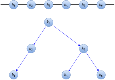
Compute the expected cost for the following binary search tree given \mathcal{D}

key	k_{1}	k_{2}	k_{3}	k_{4}	k_{5}	k_{6}
frequency	0.1	0.2	0.1	0.3	0.2	0.1

Optimal Search Cost

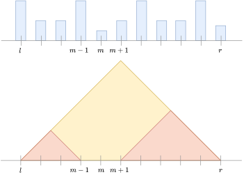
Denote \text{OptimalCost}(l,r) be optimal cost of search for a BST tree T containing \{k_{l},...,k_{r}\} given \mathcal{D}
Denote \text{OptimalCost}(l,m,r) be optimal cost of search for a BST tree T containing \{k_{l},...,k_{r}\} and k_{m} be the root node given \mathcal{D}
We have

\begin{align*} \text{OptimalCost}(l,m,r) = \sum_{i=l}^{r}f_{i} & + \text{OptimalCost}(l,m-1) \\ & +\text{OptimalCost}(m+1,r) \end{align*}

\text{OptimalCost}(l,r)=\min_{m\in\{l,...,r\}}\{\text{OptimalCost}(l,m,r)\}

Dynamic

Splay tree

A splay tree is a binary search tree with the additional property that recently accessed elements are quick to access again.

All normal operations (insert, look-up) on a binary search tree are combined with one basic operation, called splaying.
For many sequences of non-random operations, splay trees perform better than other binary search trees.

Splaying

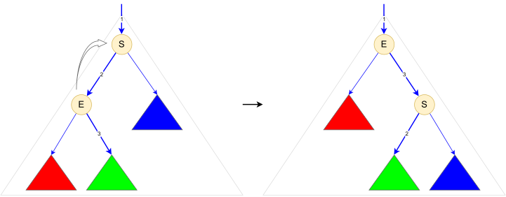
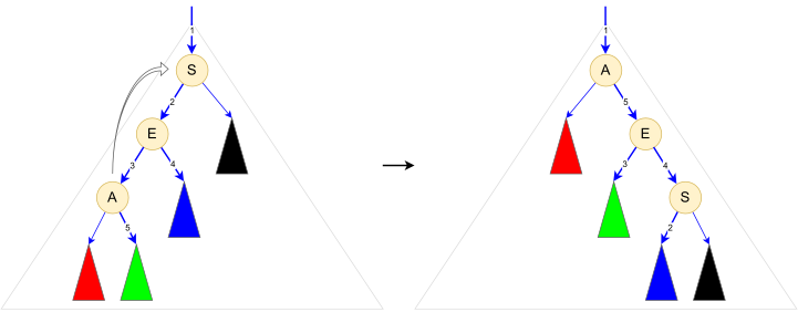
When a node x is accessed, a splay operation is performed on x to move it to the root.
To perform a splay operation we carry out a sequence of splay steps, each of which moves x closer to the root.
There are three types of splay steps, each of which has two symmetric variants:
- zig step
- zig-zig step
- zig-zag step

11.1 Balanced Tree

Introduction

Rotations

Rotations

Right rotation

Example

Implementation

Left rotation

Implementation

Strategies in Balancing Tree

Strategies in Balancing Tree

DSW algorithm

Illustration

11.2 AVL Tree

AVL Tree

The Height of an AVL Tree

Rebalancing technique

Insertion

Illustration

Deletion

Illustration

11.3 Red-Black Tree

Red-Black Tree

Example

The Height of a RB Tree

Operations

Insertion

Insertion

Example

Illustration

Deletion

Cost summary for symbol-table implementations

11.4 Optimal binary search trees

Introduction

Static

Introduction

Search Cost

Optimal Search Cost

Dynamic

Splay tree

Splaying

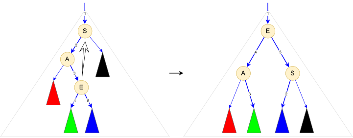
Zig step

Zig-zig

Zig-zag

11.5 Workshop

Quiz

Exercises

11.6 References