3 FRACTAL
3.1 Overview of Fractals
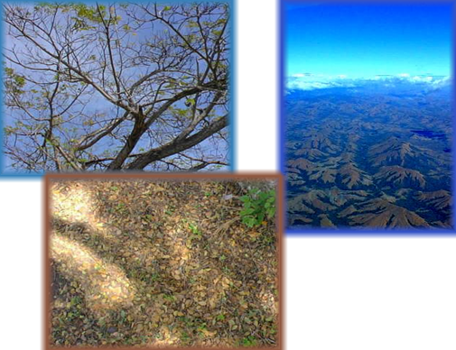
Fractal is a branch of geometry that studies objects with the property of self-similarity. This is a property where if we zoom in on a small part of the object, that part looks exactly like the whole object. This characteristic appears frequently in the natural world, such as the shapes of trees, coastlines, mountain ranges, or leaf veins.
Applications of Fractals
Fractal graphics have many practical applications:
- Image Generation: Used to create complex natural images such as clouds, mountains, water surfaces, trees.
- Image Compression: Fractal-based image compression algorithms exploit structural repetition in images to reduce storage size.
- Scientific Research: Modeling chaotic phenomena, material structures, and complex dynamic systems.
Classic Fractal Examples
Many fractals are constructed by repeatedly applying a simple generation rule:
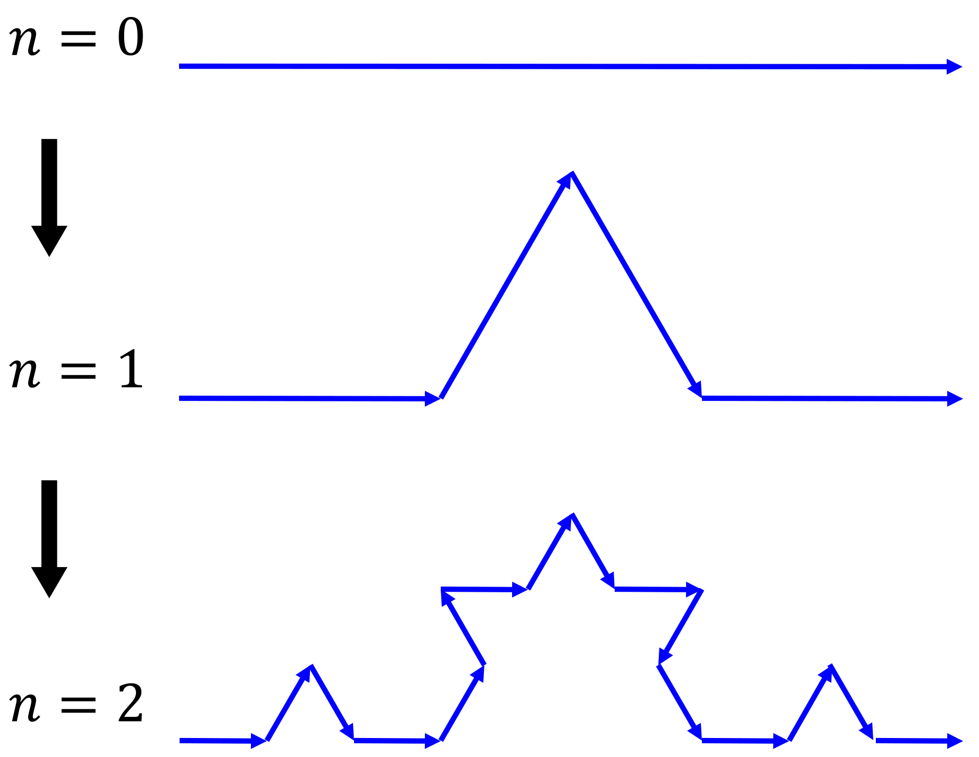
Von Koch Curve (Koch Curve):
- Base set (n=0): A line segment.
- Generation rule: Divide the line segment into 3 equal parts. Remove the middle segment and replace it with two line segments forming an equilateral triangle.
- Repetition: Apply this rule to all new line segments.
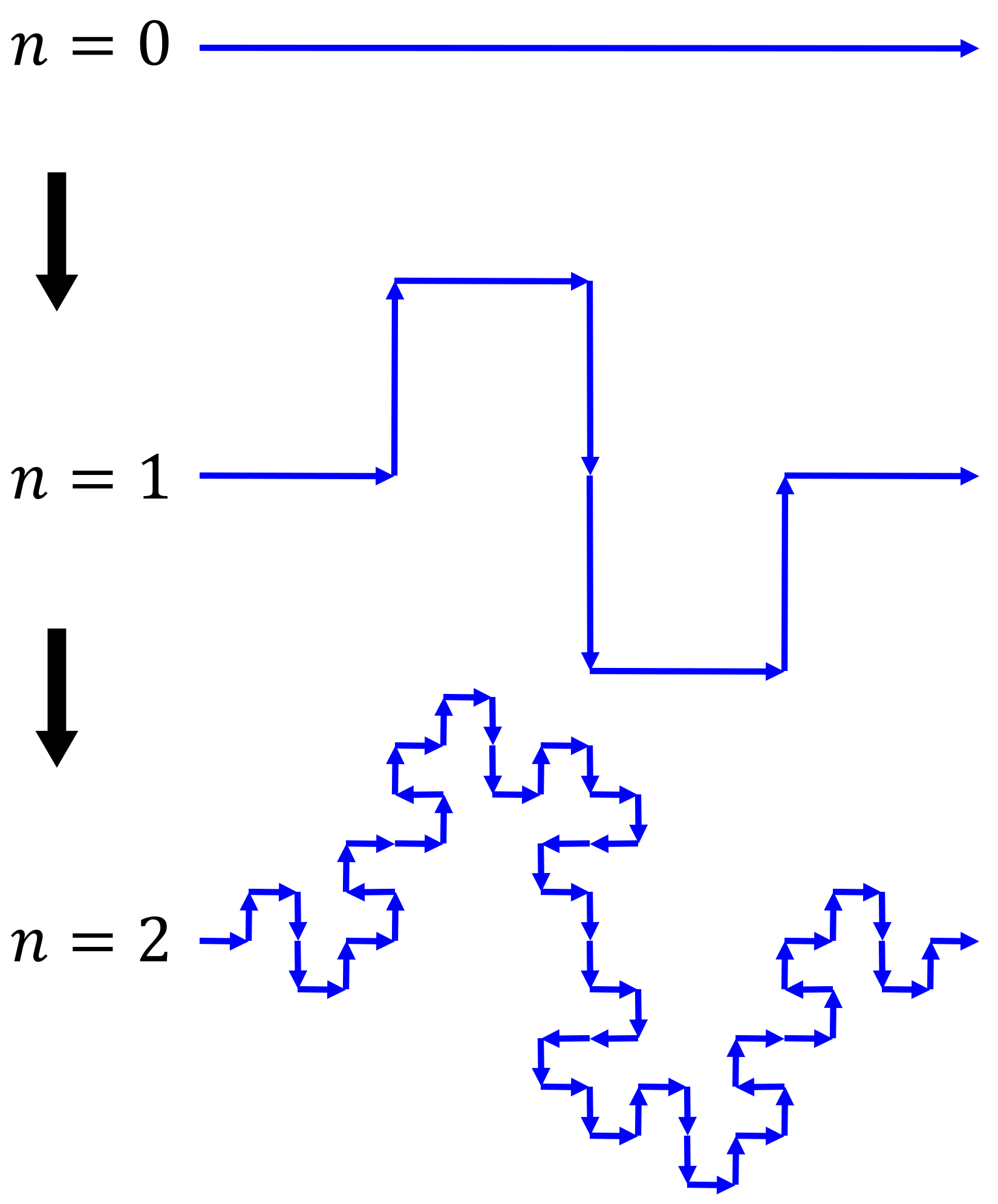
Minkowski Curve:
- Base set (n=0): A line segment.
- Generation rule: Divide the line segment into 4 parts. Remove the 2 middle segments and replace them with 6 new line segments.
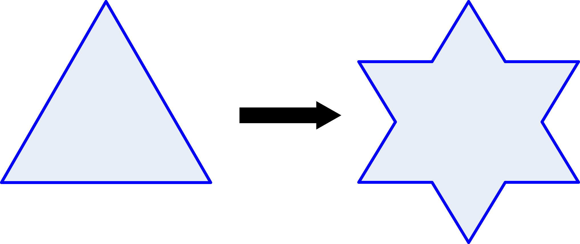
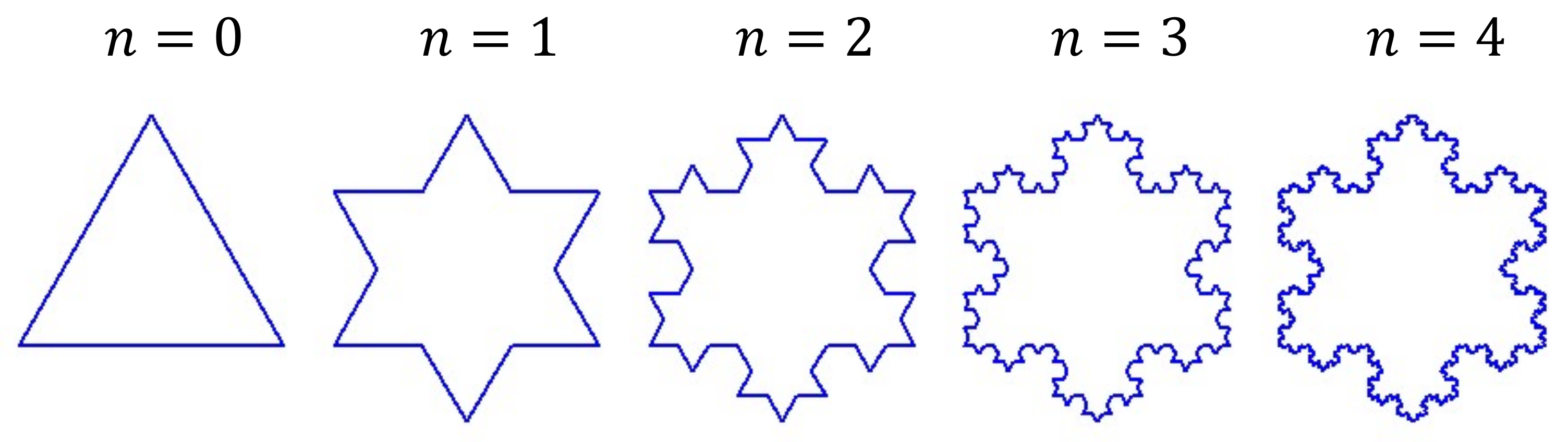
Von Koch Snowflake (Koch Snowflake):
- Base set (n=0): An equilateral triangle.
- Generation rule: Apply the generation rule of the Von Koch curve to all three sides of the triangle.
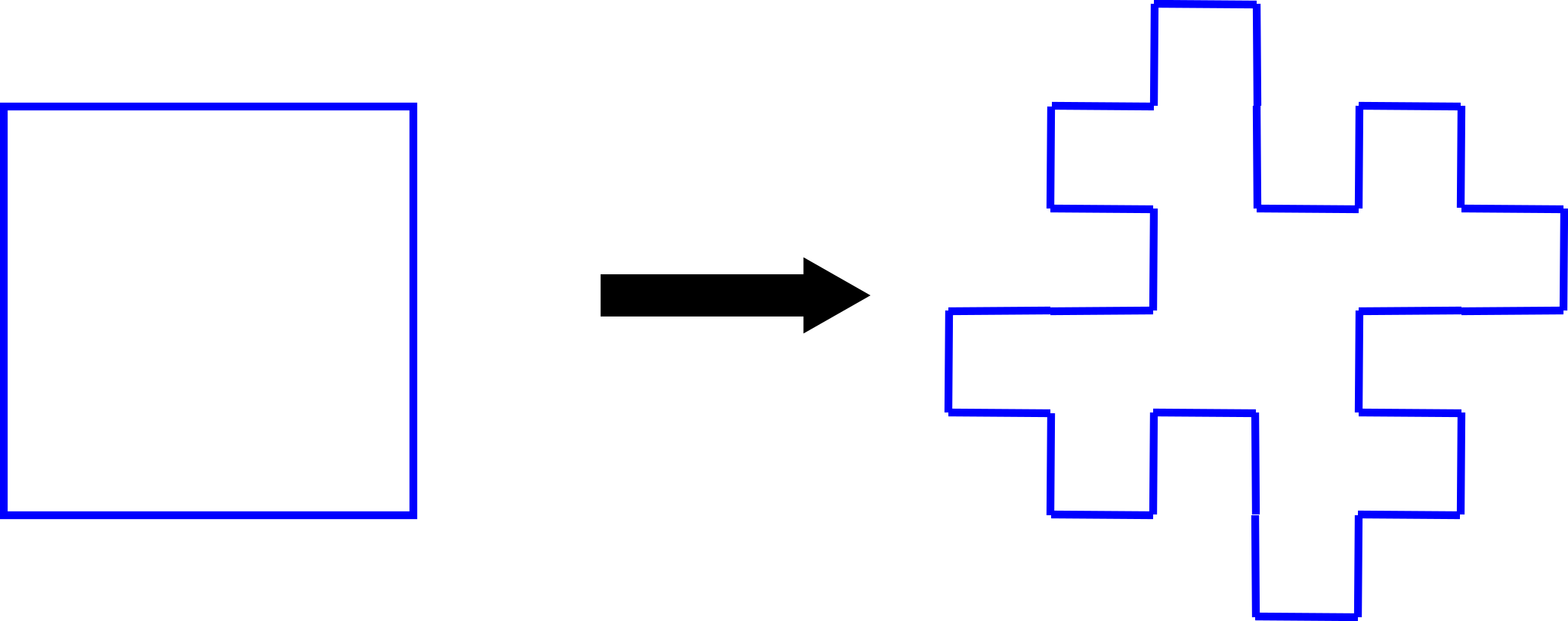
Minkowski Island:
- Base set (n=0): A square.
- Generation rule: Apply the generation rule of the Minkowski curve to all four sides of the square.
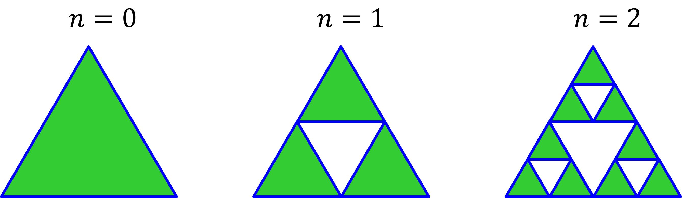
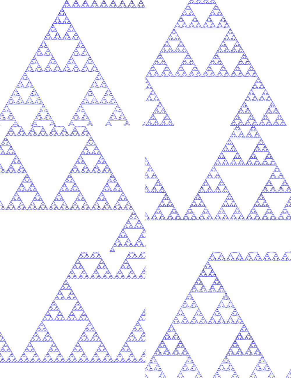
Sierpinski Triangle:
- Base set (n=0): A solid equilateral triangle.
- Generation rule: Divide the triangle into 4 smaller equilateral triangles by connecting the midpoints of the 3 sides. Remove the middle triangle.
- Repetition: Apply this rule to the 3 remaining equilateral triangles.
Fractal Dimension (Self-similarity Dimension)
An important characteristic of fractals is that their “dimension” is not always an integer (like 1D, 2D, 3D). The self-similarity dimension (D) is defined based on the relationship between the number of self-similar copies (N) and the scaling factor (s).
If a shape H is divided into N parts, each part being a copy of H scaled down by a factor s, then the dimension D is calculated as:
D = \frac{\log(N)}{\log(1/s)}
Line segment (1D): Divided into N small segments, scaling factor s = 1/N. D = \frac{\log(N)}{\log(1 / (1/N))} = \frac{\log(N)}{\log(N)} = 1

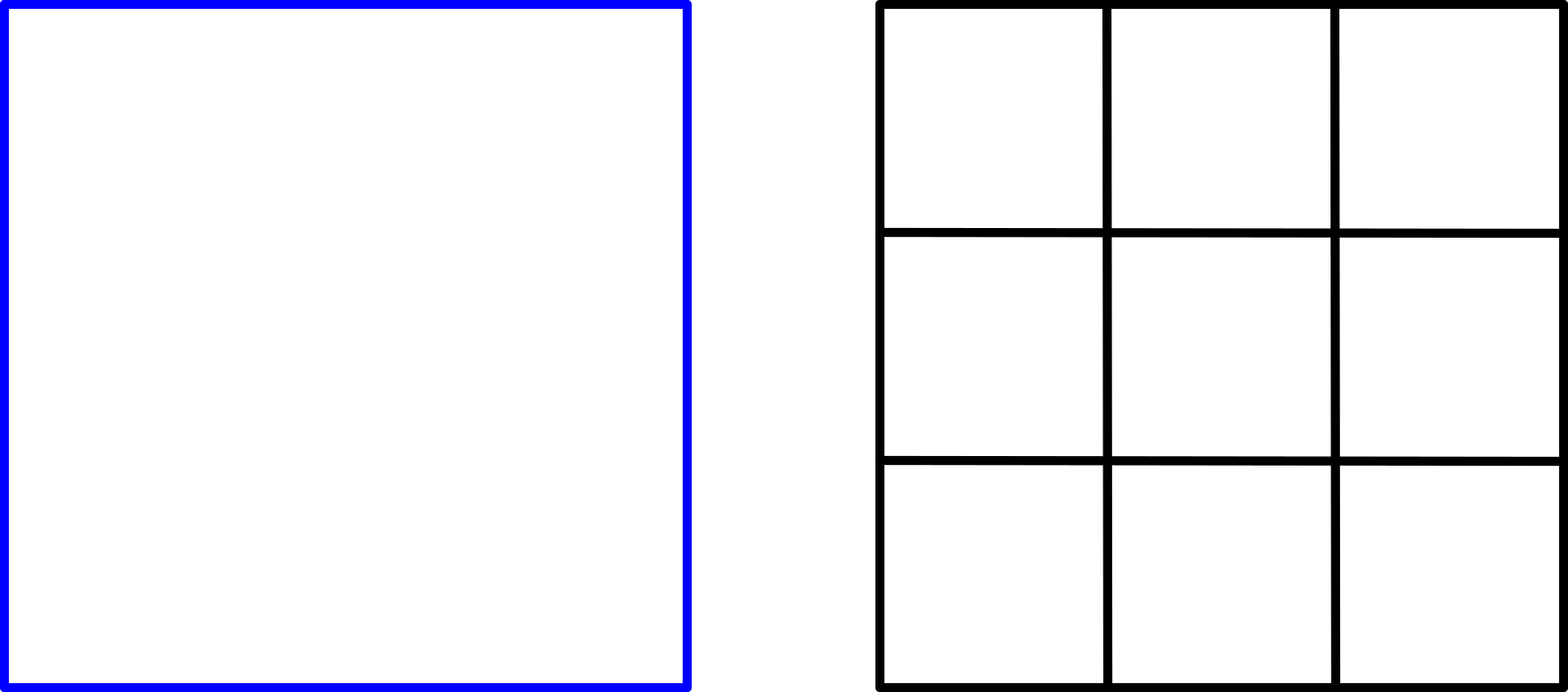
Square (2D): Divided into N \times N = N^2 small squares, scaling factor s = 1/N. D = \frac{\log(N^2)}{\log(1 / (1/N))} = \frac{2 \log(N)}{\log(N)} = 2
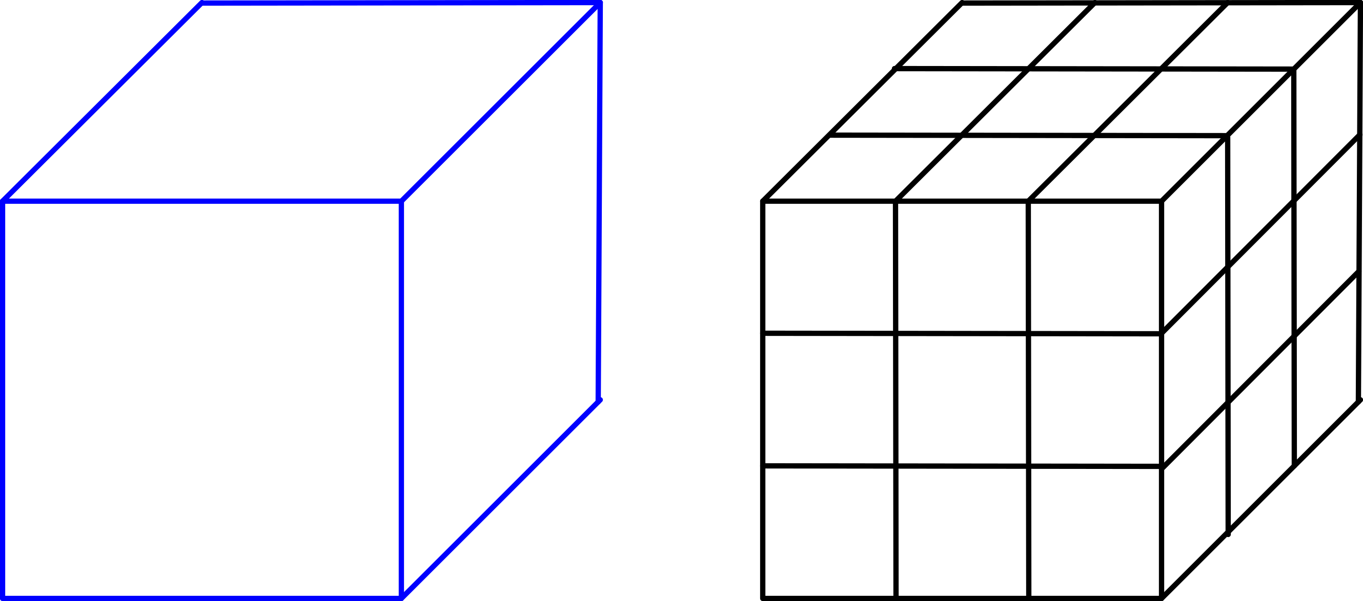
Cube (3D): Divided into N \times N = N^3 small cubes, scaling factor s = 1/N. D = \frac{\log(N^3)}{\log(1 / (1/N))} = \frac{3 \log(N)}{\log(N)} = 3
Von Koch Curve: Each segment is replaced by 4 smaller segments (N=4), each new segment has a length equal to 1/3 of the old segment (s=1/3). D = \frac{\log(4)}{\log(1 / (1/3))} = \frac{\log(4)}{\log(3)} \approx 1.26 The value 1.26 (greater than 1D of a line but less than 2D of a square) is its “fractal dimension”.

3.2 Iterated Function Systems (IFS)
IFS (Iterated Function Systems) is a solid mathematical foundation for defining and creating fractal shapes.
Mathematical Basis
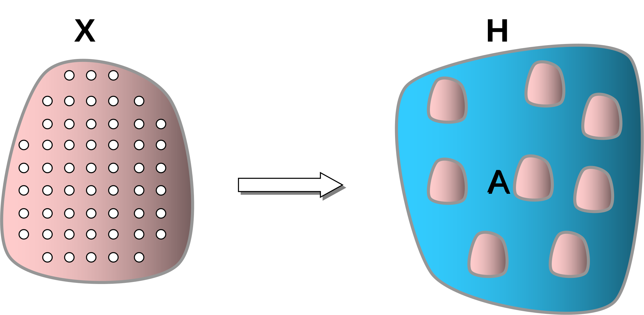
Hausdorff Space (H(X)):
- This is a special space where each “element” of it is a subset (specifically a compact, non-empty set) from X.
- One defines the Hausdorff distance h(A, B) between two sets A and B.
Contraction Mapping:
In a complete Metric space (X, d) (where we can measure distance d).
A mapping T is called a contraction mapping if it always pulls points closer together.
That is, there exists k (with 0 < k < 1) such that: d(T(x'), T(x'')) \le k \cdot d(x', x'') for all points x', x'' in X.
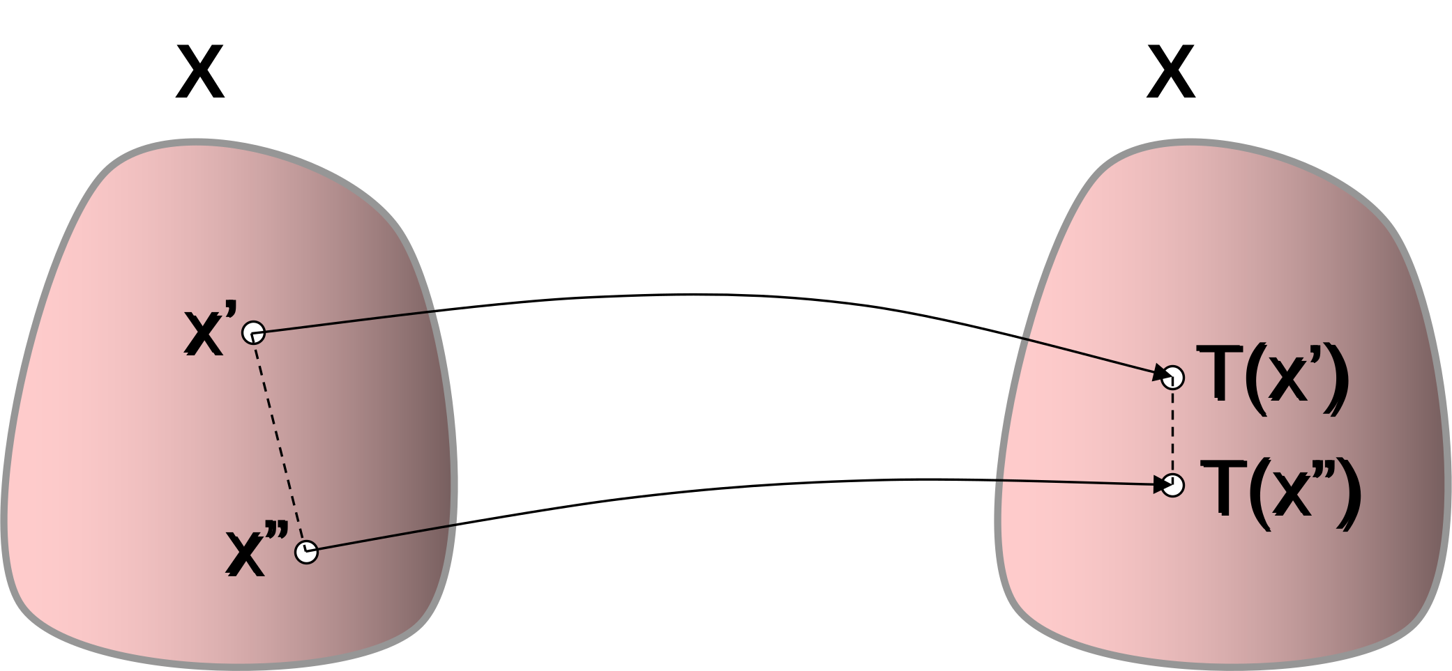
- Important Property: Every contraction mapping has a unique fixed point. If we start from any point c and iterate x_{n+1} = T(x_n), the sequence x_n will always converge to that fixed point.
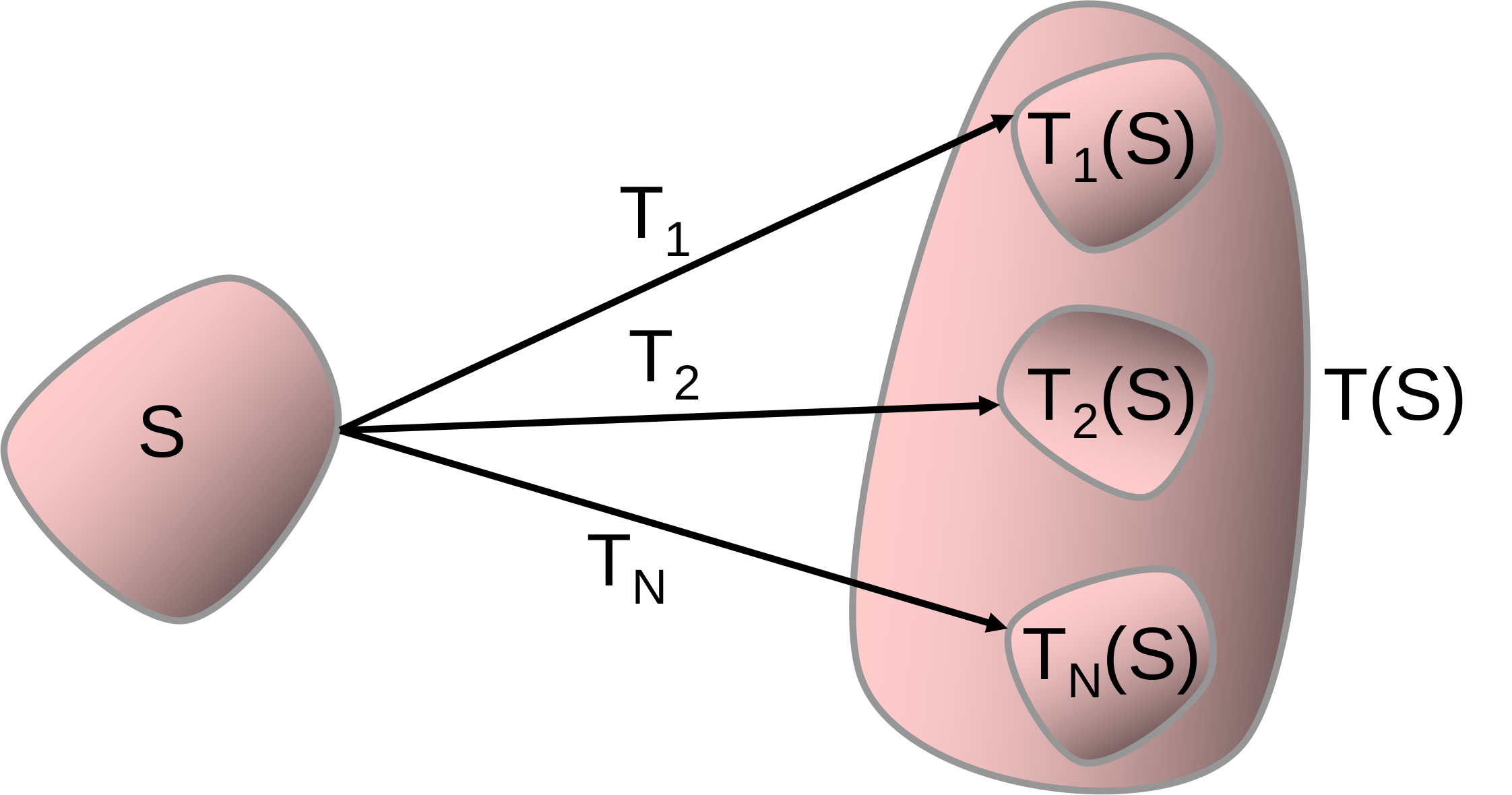
- An Iterated Function System (IFS) is a set of contraction mappings {T_1, T_2, \dots, T_N} on X.
- We define a new contraction mapping T on the Hausdorff space H(X) as follows: T(A) = T_1(A) \cup T_2(A) \cup \dots \cup T_N(A) (where T_i(A) = \{T_i(x) \mid x \in A\}).
- Since T is also a contraction mapping (in the Hausdorff space), it also has a unique “fixed point”. This “fixed point” is a set, and it is the attractor, or fractal shape, of the IFS system.
Algorithm for Generating Fractals from IFS
There are two main algorithms to draw the attractor of an IFS:
Deterministic Algorithm:
- Start with any initial shape S (e.g., a triangle).
- Iterate n times: S = T(S) = T_1(S) \cup T_2(S) \cup \dots \cup T_N(S)
- The image will converge to the fractal.
Example Equilateral Triangle (Sierpinski Triangle): Using 3 affine transformations (scaling + translation)
- T_1: Scale (0.5, 0.5)
- T_2: Scale (0.5, 0.5) + Translate (0.5, 0)
- T_3: Scale (0.5, 0.5) + Translate (0.25, 0.433)
Example Right Triangle: Using 3 affine transformations (scaling + translation)
- T_1: Scale (0.5, 0.5)
- T_2: Scale (0.5, 0.5) + Translate (0.5, 0)
- T_3: Scale (0.5, 0.5) + Translate (0.0, 0.5)
Random Algorithm:
Input: Transformations {T_1, \dots, T_N}, a starting point P_0 = (x_0, y_0), and number of iterations k.
Draw point P_0.
Loop i from 0 to k:
- Randomly select a transformation T from the IFS set.
- Calculate the next point: P_{i+1} = T(P_i).
- Draw point P_{i+1}.
After a number of iterations (e.g., k=10000), the set of drawn points will reveal the shape of the fractal.
3.3 L-System
L-System (Lindenmayer System) is a formal grammar system, originally developed to model the growth of plants. It creates fractals by string rewriting.
Turtle Graphics
L-System is often drawn using Turtle Graphics. A “turtle” (drawing pen) has 3 attributes:
- Position (p)
- Direction (\alpha)
- Drawing parameters: step size \Delta d and turning angle \Delta \alpha.
The symbols in the L-System string are interpreted as commands controlling the “turtle”:
| Command | Content |
|---|---|
| F | Move forward a segment \Delta d. |
| + | Turn the drawing pen left by an angle \Delta \alpha. |
| - | Turn the drawing pen right by an angle \Delta \alpha. |
| [ | Save the current position (p) and direction (\alpha) of the turtle (push to stack). |
| ] | Restore the saved position (p) and direction (\alpha) (pop from stack). |
L-System Definition
An L-System includes:
- Symbol Set: Characters that the turtle understands (e.g., F, +, -, [, ]).
- Axiom s_0: The initial character string.
- Production Rules: Rules for replacing characters. Example: F \to F+F-F.
Execution Process:
- Start from the axiom s_0.
- Iterate n times: At each step, simultaneously apply the production rules to all characters in the current string to create a new string (s_0 \to s_1 \to s_2 \to \dots \to s_n).
- Use Turtle Graphics to draw the final string s_n.
L-System Examples
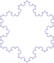
Example 1
- Axiom s_0 = F++F++F
- Production Rules
- F \to F-F++F-F
- \Delta\alpha = 60.0^\circ
Example 2
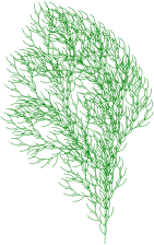
- Axiom s_0 = F
- Production Rules
- F \to FF+[+F-F-F]-[-F+F+F]
- \Delta\alpha = 22.5^\circ
Example 3
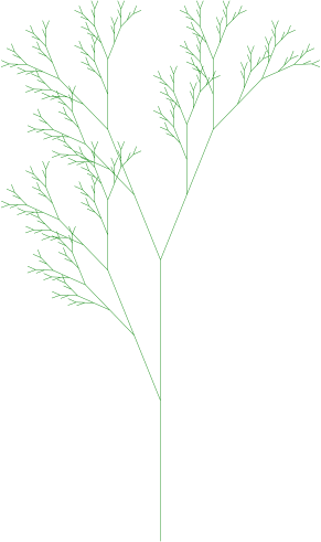
- Axiom s_0 = X
- Production Rules
- F \to FF
- X \to F[+X]F[-X]+X
- \Delta\alpha = 20.0^\circ
Example 4
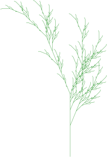
- Axiom s_0 = X
- Production Rules
- F \to FF
- X \to F-[[X]+X]+F[+FX]-X
- \Delta\alpha = 22.5^\circ
3.4 Mandelbrot Set
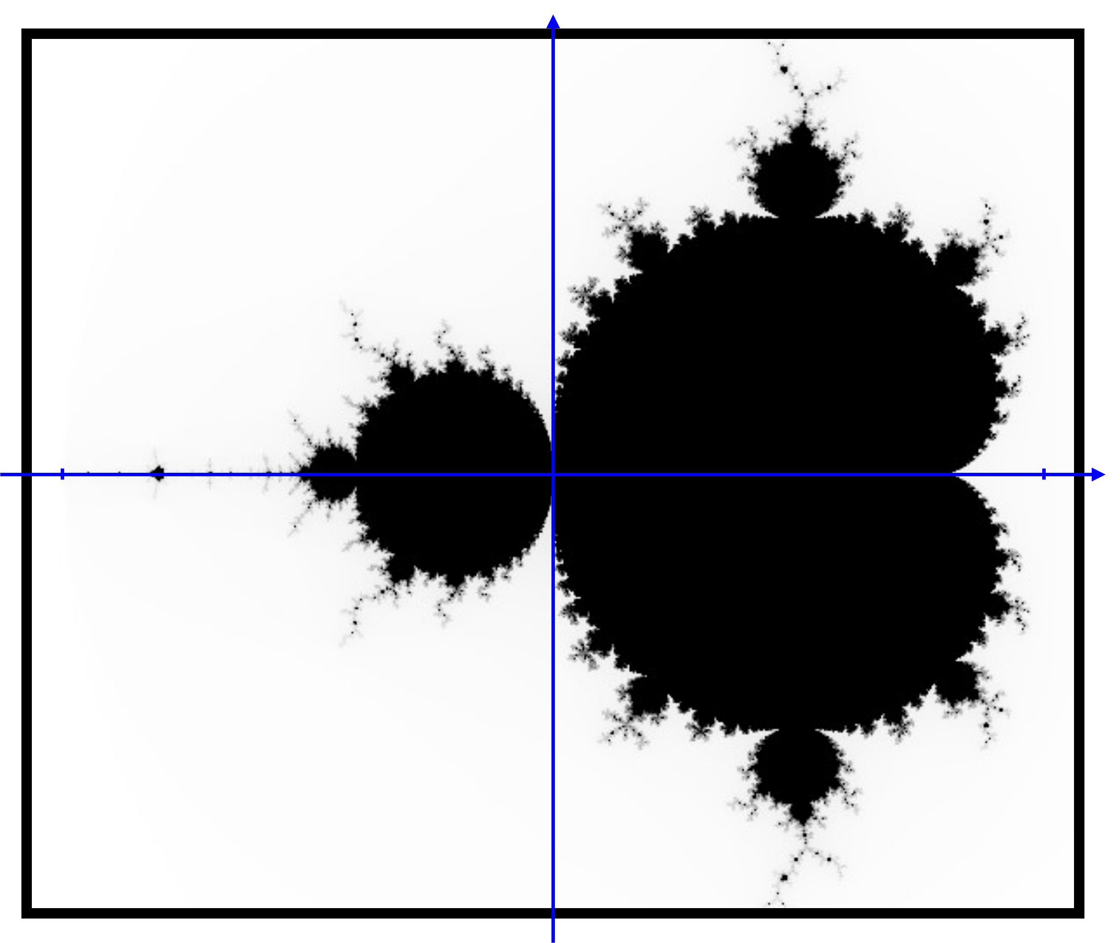
The Mandelbrot set is one of the most famous fractals, defined in the complex plane.
Definition
The Mandelbrot set is defined based on a simple recursive expression:
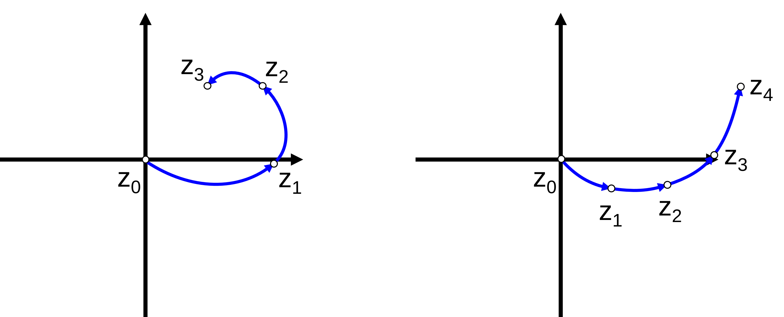
- Start with z_0 = 0 + 0i.
- Iterate: z_{n+1} = z_n^2 + c.
Where c is a complex number. The Mandelbrot set is the set of all complex numbers c such that the sequence {z_n} does not diverge to infinity (i.e., the sequence is bounded).
Convergence Property
A key property for drawing the Mandelbrot set: If there exists a k such that the modulus (magnitude) of z_k exceeds 2 (i.e., |z_k| > 2), then the sequence {z_n} will definitely diverge to infinity.
Algorithm for Drawing Mandelbrot Set
This algorithm checks each point c on the complex plane (corresponding to each pixel on the screen) to see if it belongs to the set.
For each pixel (x, y) on the screen:
Mapping: Convert pixel coordinates (x, y) into a complex number c = x + yi in a region of the complex plane.
Convergence Check:
Initialize z = 0.
Set a maximum number of iterations (e.g., N = 100).
Loop i from 0 to N:
- Calculate z = z^2 + c.
- If |z| > 2: Sequence diverges to infinity. Point c does not belong to the Mandelbrot set. Stop loop.
If the loop finishes and |z| is still \le 2: Sequence does not diverge to infinity (within the limit of N iterations). Point c belongs to the Mandelbrot set.
Coloring:
- If c belongs to the Mandelbrot set, color pixel (x, y) black.
- If c does not belong to the Mandelbrot set, do not color (leave white) (or color based on the number of iterations i before |z| > 2 to create colorful Mandelbrot images).